import pandas as pd
import matplotlib.pyplot as plt
from cdi_viz.theme import cdi_notebook_init, show_and_save_mpl

# Chapter init: resets the shared figure counter and ensures figures/ exists
cdi_notebook_init(chapter="03")

df = pd.read_csv("data/cdi-student-outcomes.csv")Matplotlib Core Skills
In the previous lesson, we focused on the question first.
Now we focus on control.
Matplotlib is not just a plotting tool.
It is a figure construction system.
If you control the figure, you control:
- clarity
- emphasis
- readability
- export quality
Initialize plotting standard
Figure vs Axes
Every Matplotlib plot has:
- A Figure (the container)
- One or more Axes (the plotting area)
Explicit control improves reproducibility.
from plotnine import (
    ggplot, aes, geom_point, geom_smooth,
    labs, theme_light, theme, element_text
)

p = (
    ggplot(df, aes(x="study_hours", y="math_score", color="test_prep"))
    + geom_point(alpha=0.55)
    + geom_smooth(method="lm", se=False)
    + labs(
        title="Study Hours vs Math Score",
        subtitle="Trend shown separately by test preparation",
        x="Study hours per week",
        y="Math score",
        color="Test prep"
    )
    + theme_light(base_size=14)
    + theme(
        plot_title_position="plot",
        plot_title=element_text(
            ha="center",
            weight="bold",
            margin={"b": 6}
        ),
        plot_subtitle=element_text(
            ha="center",
            margin={"b": 10}
        ),
        legend_position="top"
    )
)

p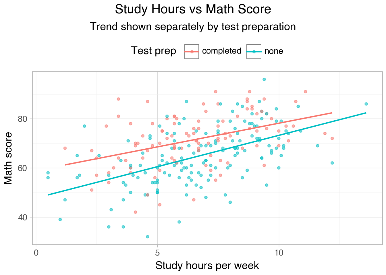
Using fig, ax is more explicit and scalable than relying on global state.
Controlling limits
Axis limits influence perception.
fig, ax = plt.subplots()

ax.scatter(df["study_hours"], df["math_score"], alpha=0.6)

ax.set_xlim(0, 16)
ax.set_ylim(0, 100)

ax.set_xlabel("Study hours per week")
ax.set_ylabel("Math score")

show_and_save_mpl(fig)  # figures/03_001.png
Saved PNG → figures/03_001.png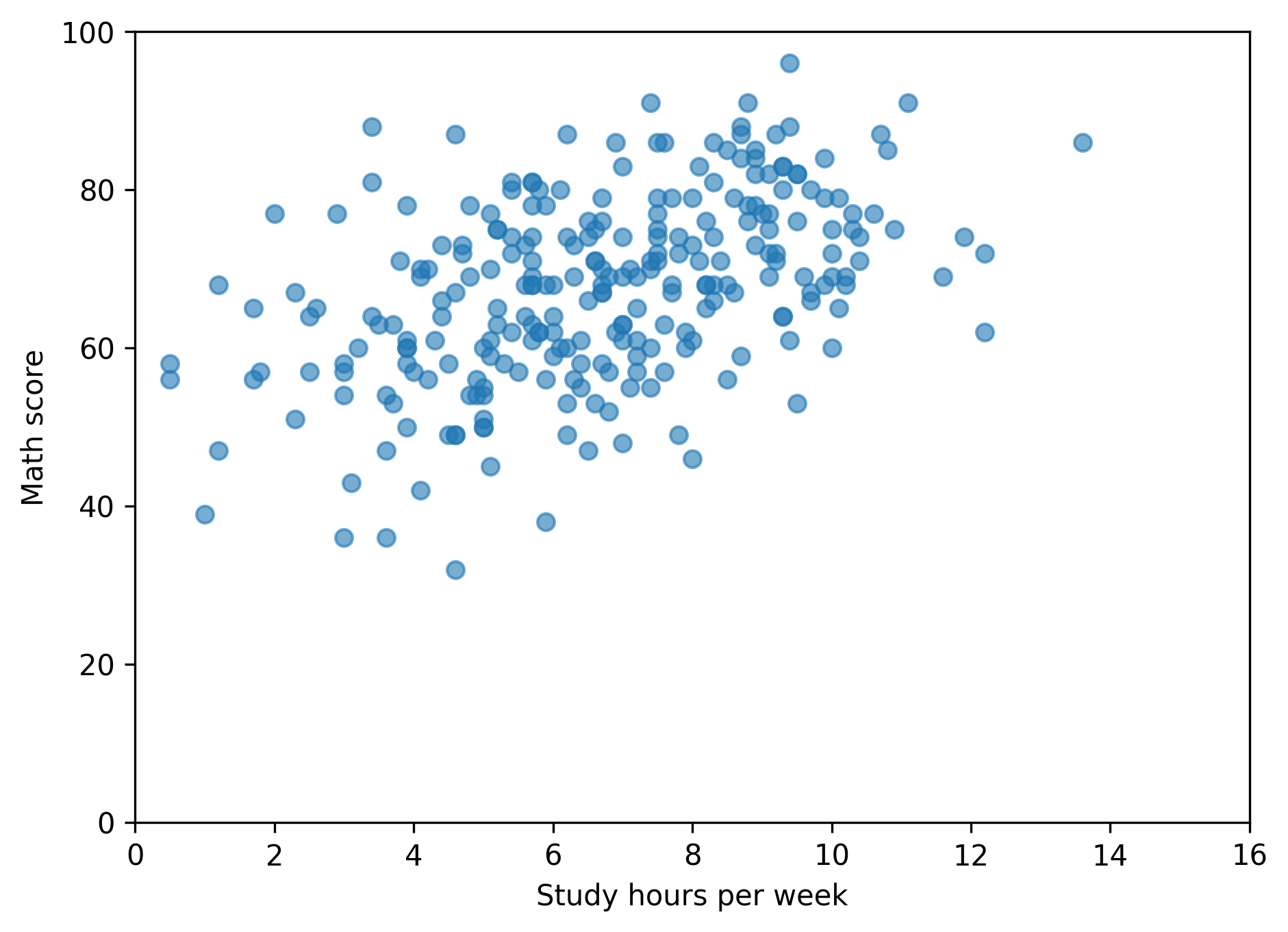
Control prevents misleading compression or exaggeration.
Adding grid discipline
Grid lines should support interpretation, not dominate it.
fig, ax = plt.subplots()

ax.scatter(df["study_hours"], df["math_score"], alpha=0.6)

ax.set_xlabel("Study hours per week")
ax.set_ylabel("Math score")

show_and_save_mpl(fig)
Saved PNG → figures/03_002.png
Subtle grids improve readability in analytical contexts.
Legends with intention
Only include a legend when grouping adds meaning.
fig, ax = plt.subplots()

for grp, sub in df.groupby("test_prep"):
    ax.scatter(sub["study_hours"], sub["math_score"], alpha=0.6, label=grp)

ax.set_xlabel("Study hours per week")
ax.set_ylabel("Math score")

ax.legend(title="Test prep")

show_and_save_mpl(fig)
Saved PNG → figures/03_003.png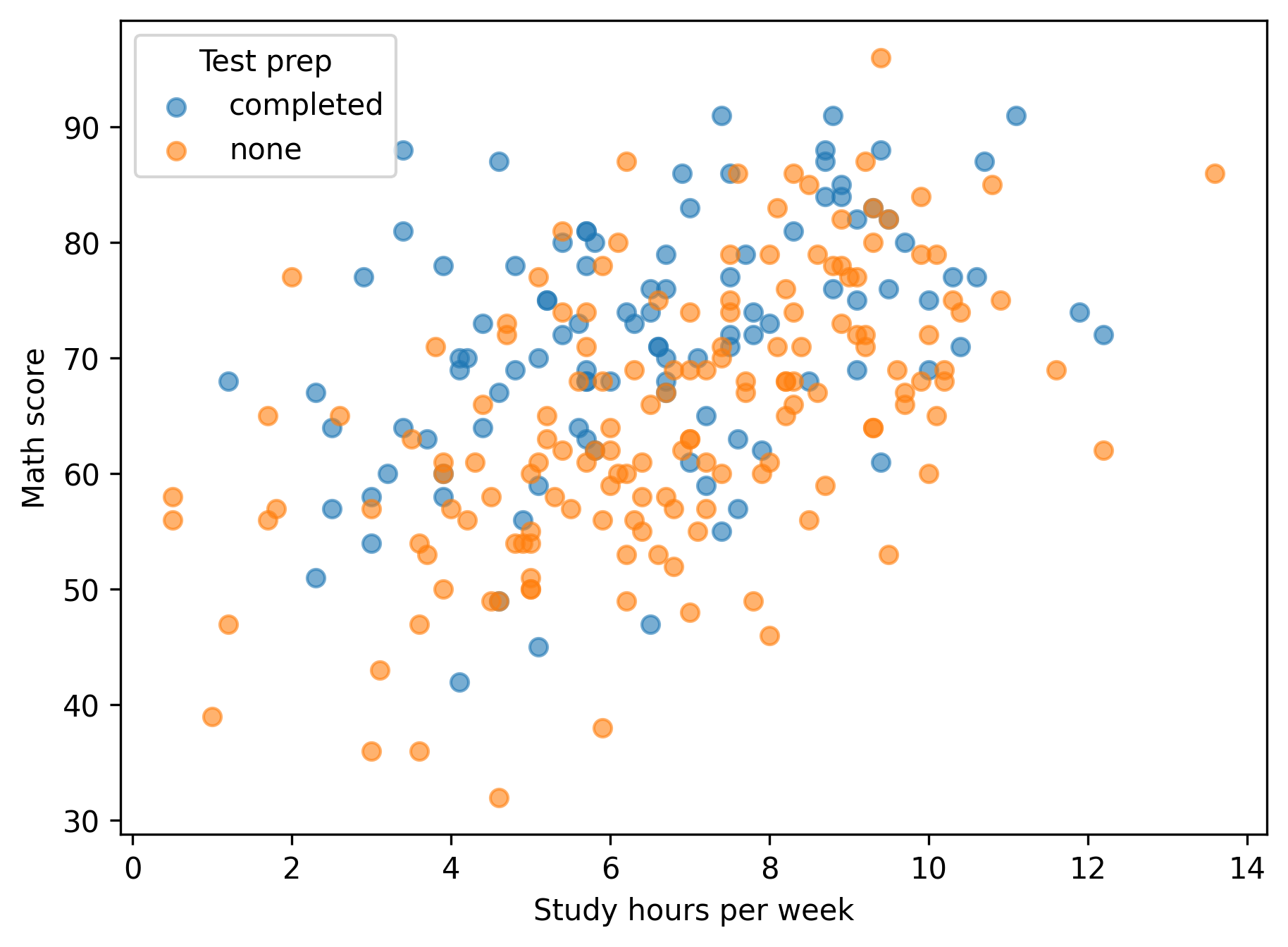
Legends clarify structure when comparisons are present.
Exporting figures consistently
Reproducibility includes export discipline.
fig, ax = plt.subplots()

ax.scatter(df["study_hours"], df["math_score"], alpha=0.6)

ax.set_xlabel("Study hours per week")
ax.set_ylabel("Math score")

show_and_save_mpl(fig)
Saved PNG → figures/03_004.png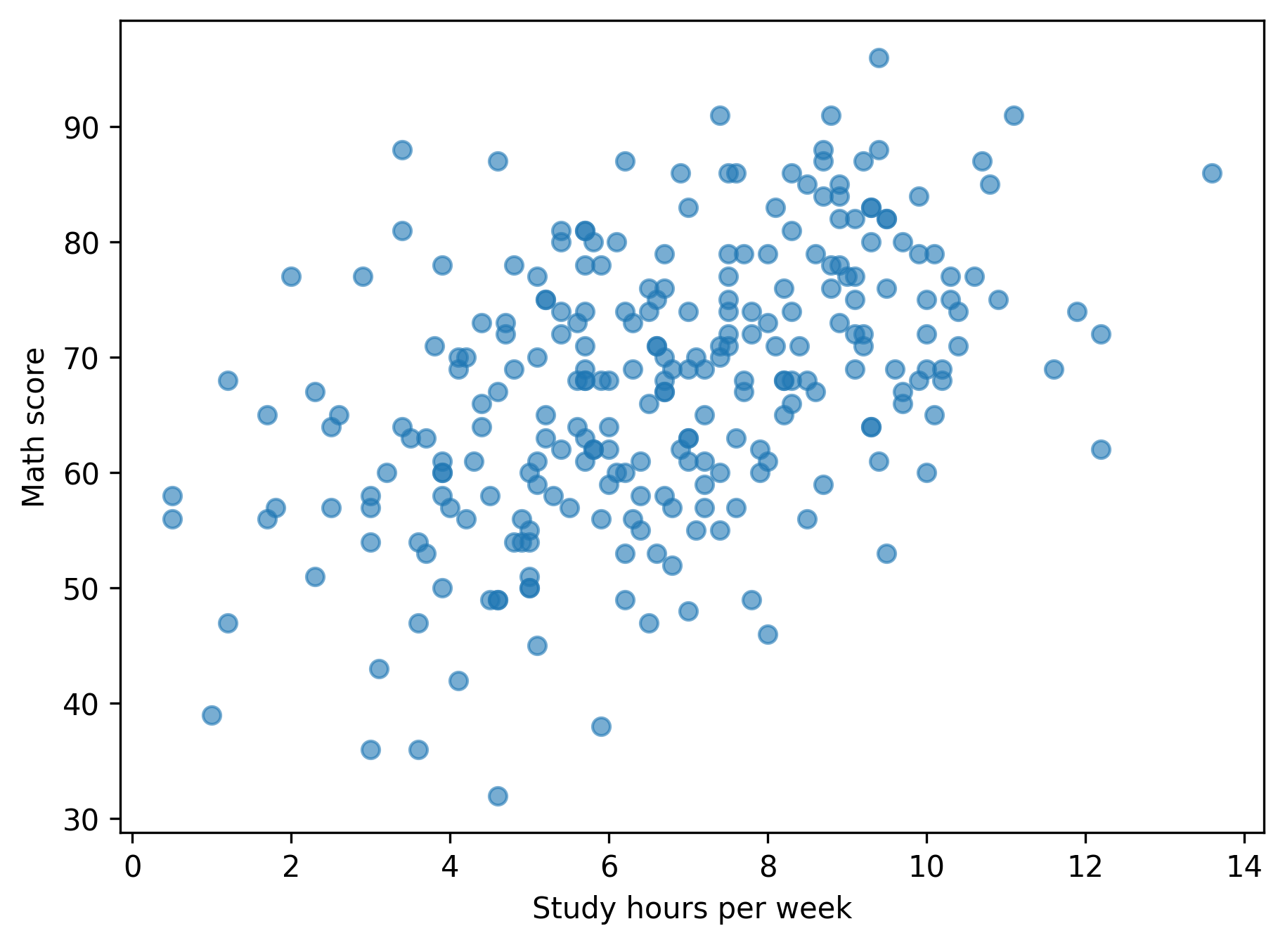
Figures are saved automatically in:
figures/03_001.png
figures/03_002.png
- etc.
Consistent naming prevents chaos in real projects.
Key Takeaways
- Use
fig, axfor explicit control. - Set labels and limits deliberately.
- Add legends only when comparisons require them.
- Export figures systematically.
- Clean structure beats decorative complexity.